An Introduction to Neural Networks: Multi-Layer Perceptrons
Neural networks are sometimes referred to as universal function approximators. This nomenclature exhibits the power and generality of neural networks which has given rise to their current popularity and success across many domains from processing and generating natural language to controlling robots and processing video streams. At a fundamental level, any neural network is a series of perceptrons feeding into one another. The perceptrons are arranged in layers with the outputs of a previous layer being the inputs into the next layer. The perceptron is therefore the fundamental building block of the neural network. We therefore suggest reading our previous article on the perceptron before delving into the details of this article.
This article was originally developed as an IPython notebook. The original code is available here on Google Colab where it can be copied and you can run and edit it yourself. Requirements for local running are available at the end of this article.
In this article, we consider the simplest case of a fully-connected network. That is a network where each node (percepton) in a given layer is connected to every node in the subsequent layer. This means that the output of a perceptron in the first layer will therefore be an input into each perceptron in the next layer. Such a network architecture is often referred to as a dense or densely connected network.
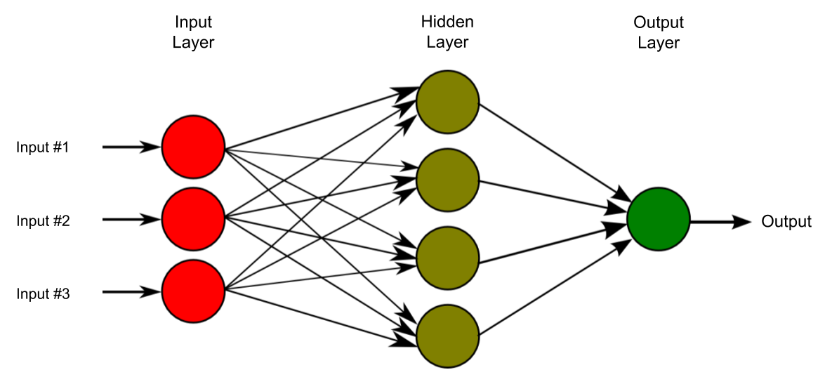
Graphical representation of a multi-layer perceptron with 3 inputs, 4 hidden units and a single output. Source: Wikimedia Commons (edited)
Building a Neural Network
In this section, we implement the neural network and a method to train the model. We first build the model by moving forwards from the inputs to the model predictions in the forward pass. We then look to train the model using gradient descent by applying the chain rule to derive backpropagation which is the key element of the backward pass. Backpropagation is the key to training all neural networks. Despite being simple, understanding backpropagation in our simple model will empower you to understand the training of any neural network.
In order to perform this modelling, we import the typical scientific data processing packages in python - numpy and pandas. We also import the plotting tools matplotlib and seaborn to collect all the imports we need in one place.
import pandas as pd
import numpy as np
import matplotlib.pyplot as plt
import seaborn as sns
sns.set()
The Forward Pass
Now that we have a problem we wish to apply our machine learner to, we need to build the learner. In the case of the multi-layer perceptrons (relatively vanilla neural networks) we will be using here this is relatively simple.
If one is familiar with summation notation and matrix algebra the mathematics and implementation of the forward pass is surprisingly simple for such a powerful model. The formula for prediction is given below where \(w_{i, j}\) denotes the weight from node \(i\) to node \(j\), \(w_{0, \cdot}\) denotes the bias in the respective layer, \(output\) denotes the output node, the \(i\)'s range over the inputs (of which there are \(n_{input}\)) and the \(j\)'s range over the nodes in the hidden layer (of which there are \(n_{hidden})\).
$$prediction = w_{0,output}+\sum_{j=1}^{n_{hidden}} w_{j,output}\cdot \sigma\left(w_{0,j}+\sum_{i=1}^{n_{input}} x_i w_{i,j}\right)$$
One memorable way of phrasing the operations of each layer in a neural network works, (to my knowledge) coined by Siraj Raval, is as below.
Input times weights, plus a bias, activate!
Put mathematically, take the matrix product of your vector of inputs and the matrix of weights for the layer in question, add a bias and pass the result through your chosen activation function. The matrix form of the forward pass is written below where \(W_k\) denotes the weights matrix for layer \(k\) and \(b_k\) denotes the bias vector for each layer. In writing this equation we assume that the activation function (denoted by \(\sigma\)) is applied elementwise to vector arguments (i.e. is vectorised).
$$prediction = \boldsymbol{b_2} + \boldsymbol{W_2}\left( \sigma\left(\boldsymbol{b_1} + \boldsymbol{W_1}\boldsymbol{x}\right)\right)$$
Note that, for non-input layers, the inputs are the outputs of the previous layer and that, in practical implementations, adding a bias is usually done by prepending a 1 to the start of your input vector and adding another row (the biases) to the top of the weights matrix. This then deals with adding the bias through the matrix multiplication. Element \((i, j)\) of any given weight matrix (usually denoted \(w_{i,j}\)) is the weight of the \(i^{\text{th}}\) input element in the sum to calculate the value of node \(j\) (in the subsequent layer).
In order to check that you understand the above equations, think about how they would change if our network had two hidden layers instead of one.
Activation Functions
Activation functions determine how a perceptron produces its output. Unlike neurons, perceptrons are not limited to binary output and hence may produce any real number as their output. The choice of activation function can therefore shape this output by shaping the relationship between inputs and the output beyond the linear way in which weights enter the equation. This relationship change can be made for computational ease, to match the relationship we are trying to estimate or to aid in training the model. By introducing some non-linearity to the operations of a neural network, an appropriate choice of activation function can greatly improve the expressiveness of a neural network.
In the case of the neurons in our brains that the perceptrons aim to emulate, activation functions play the role of the activation threshold which modulates the rate and timing of the firing of neurons. In the brain the threshold is placed on a concentration gradient across a membrane which much reach a certain strength before an activation potential will be passed along the neuron. In our case, working in the mathematics of real numbers we may consider the output as any value on the real domain. This can be considered the number of action potentials per second should one wish to maintain the biological parallel.
The Sigmoid Function
A binary classifier may aim to place a probability on the given input belonging to a given class. This will mean that the outputs must, by way of being probabilities, fall in the unit interval \((o \in [0,1])\). The sigmoid function will always produce outputs that are between 0 and 1 and can therefore be considered to produce valid probabilities. In other cases, the sigmoid function may be used to add some non-linearity to the calculations whilst also containing the values to a known and standard scale. Our example neural network here is a case of the latter where we do not need probabilities but are implementing a neural network in its simple first incarnation. Today, other activation functions, such as the ReLU, are more popular but the intuition and the mathematics carries over.
The functional form of the sigmoid function is given below.
$$\sigma(x)=\frac{1}{1+e^{-x}}$$
Note that this function is strictly increasing in \(x\) and varies from \(0\) when \(x\) is \(-\infty\) and \(1\) when \(x\) is \(\infty\). It is smooth, defined for all real numbers and differentiable everywhere.
In fact, the differential takes a rather nice form which is one reason for the function's popularity. This will help us when training the model later on.
Let's plot the sigmoid function so that we can see what we're dealing with.
First, we define our sigmoid function. Note that we decorate it with numpy's vectorize function so that the function can be called on lists and arrays without further modification.
@np.vectorize
def sigmoid(x):
    return 1/(1+np.exp(-x))
Finally, let us generate some points and create a plot.
x = np.linspace(-10, 10, 1000)
y = sigmoid(x)
plt.plot(x,y, figure=plt.figure(figsize=(9,4.5)))
plt.axvline(0, color='k', lw=0.5)
plt.xlabel('$x$', size=15)
plt.ylabel('$\sigma(x)$', size=15);
We now turn to the derivative of the sigmoid function.
Training of neural networks requires following the gradient of an objective function. This requires the model to be differentiable which in turn means that the activation functions need to be differentiable. Let us find the differential of our sigmoid activation by applying the quotient rule.
$$\frac{d\frac{u}{v}}{dx}=\frac{v\frac{du}{dx} - u\frac{dv}{dx}}{v^2}$$
This leads us to the following derivative of the sigmoid function.
$$ \begin{align} \sigma'(x) &=\frac{e^{-x}}{(1+e^{-x})^2}\\&=\frac{1}{1+e^{-x}}\cdot \frac{e^{-x}}{1+e^{-x}}\\&=\frac{1}{1+e^{-x}}\cdot\frac{(1+e^{-x})-1}{1+e^{-x}}\\&=\frac{1}{1+e^{-x}}\cdot\left(1-\frac{1}{1+e^{-x}}\right)\\&=\sigma(x)(1-\sigma(x)) \end{align} $$
We may now plot the derivative of the sigmoid function to consider how its selection as the activation function in our network could affect training through gradient-based methods
y = sigmoid(x) * (1 - sigmoid(x))
plt.plot(x,y, figure=plt.figure(figsize=(9,4.5)).set_dpi(400))
plt.axvline(0, color='k', lw=0.5)
plt.xlabel('$x$', size=15)
plt.ylabel("$\sigma'(x)$", size=15);
We may see that for inputs of large magnitude the derivative of the sigmoid function is very small. This is clear from its functional form. The \(\sigma(x)\) term tends to zero as \(x\) increases and the \(1-\sigma(x)\) term tends to zero as \(x\) becomes increasingly negative. The largest value the gradient can be is \(0.25\) when \(x\) is zero. As we will see later, training a neural network requires following gradients. Therefore, small gradients can hamper training. The case where changes in the arguments to an activation function have very little influence over the output of the activation function is known as saturation of the activation function. This occurs for very high and very low argument values in the case of the sigmoid function. Avoiding such saturation points, which inhibit learning, is one reason why we initialise the weights of a neural network to random small values at the start of training.
Generating Predictions
In the network we are building, we select the sigmoid function as our activation function. This limits the outputs of the given layer to be in the unit interval. However, we know from the data generation work above that the outputs will not necessarily be in this interval. Therefore, in the final layer, in order not to limit the range of outputs, we will apply no activation at all. This changes the formula above by taking out the sigmoid transformation \((\sigma(\cdot))\), this can also be considered by just changing the activation function in the final layer to an identity function \((f_{identity}(x) = x)\).
Given the formulae above, we can write our prediction function. It takes the input vector \(\boldsymbol{x}\) and a list of weight matrices (one for each layer of the neural network) and conducts the arithmetic above.
Initially a \(1\) is inserted in the first position of the input vector \(\boldsymbol{x}\) to account for the bias (included here as an extra row of weights in the relevant weight matrices). Then for each intermediate (i.e. 'hidden') layer the matrix multiplication is conducted and the activation function applied to this output. To again account for an additive bias, a \(1\) is prepended to the hidden layer output vector. Note that the final layer, having no activation function, is treated separately on the penultimate line of the function written below. The matrix multiplication is carried out as normal, yet no activation is applied.
def predict(x, weights):
    x = np.insert(x, 0, 1)
    output = x
    for layer in weights[:-1]:
        output = sigmoid(np.matmul(output, layer))
        output = np.insert(output, 0, 1)
    output = np.matmul(output, weights[-1])
    return output
Let us run a quick test example of how this prediction function works to make sure all is working well before we develop our training algorithm.
Walking through the Forward Pass
For a working example we need weights and some input. We will initialise the weights to be small random numbers. These are the weights we will start to learn from later on and hence we do not wish to include any big values as to do so imposes some strong prior view as to the relationship between the inputs and outputs and particularly large values may risk saturating the sigmoid activation function.
The weights for each layer will be stored in an \(n\times m\) matrix where \(n\) is one greater than the number of nodes in the previous layer (one greater to account for the bias to be added) and \(m\) is the number of nodes in the subsequent layer (this time ignoring any bias 'node').
w = [
        np.random.normal(0, 0.5, size=(5,5)),
        np.random.normal(0, 0.5, size=(6,1))
    ]
Since the relationship we are learning has been developed here for pedagogic reasons, it it not necessarily meaningful as our focus is on the mathematics of modelling. Therefore, we can choose any values from the ranges included in the inputs.
x = np.array([0.003, 0.19, 0.1, 0.39])Finally, we can run our prediction with our chosen inputs and the random weights. Note that the output is a 1-vector (a numpy array) rather than a raw scalar value, since it is the result of matrix multiplication. This means that the network can be generalised to have multiple outputs.
predict(x, w)array([-0.3672341])
Should you wish to consolidate your understanding of how this network works, the list of weight matrices is given below so that you may trace and check the calculation yourself by hand, outside of Python.
print(w)[array([[-0.35488876, -0.23659869, -0.33867314, 0.36387468, 0.32611655],
[-0.26065506, -1.05467748, 0.18559385, 0.25842844, -0.40552946],
[-0.08049153, -0.62635345, 0.52101412, -0.08069795, -0.83872539],
[-0.72111432, -0.29579596, -0.27537176, 0.66396855, 0.20578943],
[ 0.52081198, -0.68363231, 0.01350068, -0.11467529, 0.26864561]]),
array([[ 0.03878111],
[ 0.70394749],
[-0.84874312],
[ 0.50273702],
[-0.8350314 ],
[-0.26286314]])]
Setting a Problem to Solve
To consider how neural networks work, we need a set of data to learn from. In this article, we will consider a regression problem for which the outcome is determined by some non-linear function of the inputs. This non-linear function is what we aim to learn with our network and is chosen such that it reflects the inner workings of our network. The complexity of having a non-linear function to learn means that this problem is beyond the capacity of a single perceptron which learns a linear function.
First, we must consider the relationship we wish to build. Let us consider a function of 4 variables. We will then build a network with one hidden layer of \(5\) units to approximate the true function.
We let our input variables be random normal values \((a, b, c, d \sim \mathcal{N}(0,1))\) so that values are all on a standardised scale. This aids in the training of the network. While this scaling wont necessarily be the same in real data sets data is usually normalised (yielding so-called z-values) before training a neural network with it. The reason for normalisation is to achieve a consistent order of magnitude of the inputs which prevents values very large in magnitude from being realised which would saturate the activation functions. Furthermore, a consistent scale of values across problems makes hyperparameter selection and tuning more general across problems. We can save the values used in the original normalisation (the mean and the standard deviation of the training data) so that other data (e.g. the test set) can be standardised in exactly the same way.
We start by generatng some data.
a = np.random.uniform(size=10000)
b = np.random.uniform(size=10000)
c = np.random.uniform(size=10000)
d = np.random.uniform(size=10000)
Now let us define a function of these variables which we will learn to approximate with a neural network.
@np.vectorize
def hyperplane(a,b,c,d):
    value = sigmoid(0.1*a) + 0.4*sigmoid(b) - 0.2*sigmoid(c) + sigmoid(d)
    return value
We apply this function to attain the outputs we will later seek to predict. We will refer to these as the true values as they are generated by the process we wish to learn. They are stored in the variable true_values accordingly.
true_values = hyperplane(a,b,c,d)Finally, we put all of our data in one place. We generate a dataframe with the inputs having their own columns and the outputs appended on the right. This is similar to how we may expect a real data set from an experiment to look. Working with pandas should aid transition to any other work you may wish to pursue with neural nets (particularly if using the standard introductory machine learning package scikit-learn).
dataset = pd.DataFrame(data={
    'a':a,
    'b':b,
    'c':c,
    'd':d,
    'value': true_values
})
A quick peek at the data set to finalise the data initialisation and save us rereading this section when we wish to quickly understand the structure of our data set.
dataset.head()| a | b | c | d | value | |
|---|---|---|---|---|---|
| 0 | 0.915241 | 0.876958 | 0.505173 | 0.072895 | 1.198823 |
| 1 | 0.651209 | 0.839387 | 0.396698 | 0.127875 | 1.207955 |
| 2 | 0.560437 | 0.257284 | 0.839789 | 0.385774 | 1.195175 |
| 3 | 0.680295 | 0.022301 | 0.435102 | 0.412747 | 1.199559 |
| 4 | 0.282659 | 0.047266 | 0.276772 | 0.855818 | 1.299827 |
Training a Neural Network
Similarly to the case of the vanilla perceptron we considered in a previous article, the values passed as inputs to each layer (and therefore each perceptron in that layer) will have weights associated with them. These weights are the variables which are updated during training with the goal of loss minimisation.
In contrast to a single perceptron, training a multi-layer perceptron can appear more complex since the weights in the first layer only have an indirect impact on the output via multiple paths. We will see, however, that training a neural network typically boils down to applying the chain rule to matrix equations.
The indirect influence of any given input on the network's output is difficult to trace in the case that the activation function is a step function (as was the case in the single perceptron). The discontinuous step function is not differentiable everywhere, at the point of discontinuity the derivative is not defined and elsewhere the derivative is zero. This means that we cannot calculate the gradient of the error to follow to descend the loss. Gradient descent in the loss for the weights of a neural network is known as backpropagation as the training signal (the gradient of the loss) is propagated backwards through the network to all of the trainable weights. We consider this process in detail below.
In order to undertake backpropagation the error, and so in turn the model prediction, needs to be differentiable with respect to the weights. In order to achieve this, a smooth (differentiable) activation function is used in place of the perceptron step function.
We discuss the mathematics of backpropagation below.
The Backwards Pass: Backpropagation
Now comes the more mathematically involved part. Training the model.
The forward pass, presented above, is also known as forward propagation as the calculation at each stage is propagated forwards into the next calculation. For the model to learn, it must learn from the errors in its outputs. These errors are the differences between the predictions and the known values. The errors can only be calculated at the end of a forward pass. However, the parameters we wish to update in order to reduce the error (namely the weights in each layer) occur earlier in the calculation. Training therefore requires that the errors and information from later layers be passed back to layers closer to the inputs to in the network ('earlier' layers). This led to the backpropagation algorithm whereby the errors and information from later layers are used when training a given layer.
Before we lay out the mathematics of the training algorithm, let us first consider the intuition of the training process. We will define a loss function that is proportional to the prediction error (but may contain other penalties or weight certain errors more heavily than others). This loss function will be defined over all possible values for the weights in our model. The aim is therefore to minimise the loss function (thereby reducing prediction errors) by updating the weights within our neural network.
The approach we will take is gradient descent. The intuition is as follows: Imagine that there are only two weights over which you wish to minimise the loss. The loss is therefore defined at all possible pairings of weight values. Given that the weights are continuous variables, the space of weights and the related losses can be plotted in three-dimensional space with the 'floor' being coordinates in \(w_1, w_2\) space and the height at any point being given by \(loss = L(w_1, w_2)\). We can imagine this to resemble a mountainous landscape. The weights are initialised at a random point \((w_1^{start}, w_2^{start})\) from which we wish to get to the optimum \((w_1^*,w_2^*)\) which will be the lowest point on the surface (i.e. the point where the loss is minimised). Mathematically, we are looking to find \(\text{arg}\min_{(w_1,w_2)}{L(w_1, w_2)}\). We will get there step by step by moving 'downhill'. This is done by calculating the gradient at our current position, the direction of steepest descent, and then taking a step of given size in that direction. After this step we re-evaluate the gradient and then continue on with another step. This descent will bring us down until we reach a minimum or we run out of steps or compute time.
Note that in the above we end at a minimum which is not necessarily the global minimum. The problem of arriving at a local minimum is one that is greatly explored in all optimisation. This, alongside problems around overfitting, choosing the step size and many more elements of designing and implementing an optimisation algorithm, will be left for discussion in future articles. Here, we focus on the mathematics of our chosen optimisation algorithm. The key to gradient descent is finding the gradient we wish to take a step in the direction of. This gradient (of the loss function) is given by the vector below.
$$\nabla L(\boldsymbol{w}) = \left[\frac{\partial L}{\partial w_{0,1}}, \frac{\partial L}{\partial w_{0,2}}, \cdots, \frac{\partial L}{\partial w_{n_{hidden},output}}\right]$$
Now we may define the loss function and find its derivative. Once we have this information we will be able to train our multi-layer perceptron.
We will use a simple standard loss function of minimising the sum of squared residuals. We will scale this loss to make some of the later mathematics easier. We define the loss across all data points \(d\) in the available data set \(D\) as below.
$$Loss = \frac{1}{2} \sum_{d\in D} \left(\hat{y}_d - y^{\ true}_d\right)^2$$
Where the model prediction is given by \(\hat{y}\) and the target value is given by \(y^{\ true}\).
Now that we have the loss function along with a formula for the prediction as a function of the weights, we may take derivatives to build up the gradient vector.
First, let us remind ourselves of the forward pass formula.
$$prediction = w_{0,output}+\sum_{j=1}^{n_{hidden}} w_{j,output}\cdot \sigma\left(w_{0,j}+\sum_{i=1}^{n_{input}} x_i w_{i,j}\right)$$
At a high level, the derivative of the loss function with respect to some weight \(w_{i,j}\) will be given by the following.
$$\frac{\partial Loss}{\partial w_{i,j}} = \sum_{d\in D} \left(\frac{\partial \hat{y}_d}{\partial w_{i,j}} \left(\hat{y}_d - y^{\ true}_d\right)\right)$$
Note that the \(\frac{1}{2}\) we scaled the loss by cancels with the power of \(2\) when we take the first derivative, this saves us from juggling constants without losing anything of consequence.
The non-trivial part of this derivative is the term in the derivative of \(\hat{y}\). Let's focus on this term and rebuild the full derivative once we have all the parts.
Let us consider the simpler case of an element of the final layer (i.e. this derivative for weights between the hidden layer and the output).
$$\frac{\partial\ \hat{y}}{\partial w_{j, output}} = h_j$$
Where \(h_j\) denotes the value of the \(j^{\text{th}}\) unit in the hidden layer and \(w_{j, output}\) denotes the weight between the \(j^{\text{th}}\) node of the hidden layer and the output node. To clarify:
$$h_j = \sigma\left(w_{0,j}+\sum_{i=1}^n x_i w_{i,j}\right)$$
The more complex derivatives are those concerning the weights earlier in the tree. This makes sense as they do not affect the prediction so directly as they influence the values in the hidden layer which then affect the output through another layer of calculation. Therefore, these weights have a derivative for the prediction depending on more terms. This derivative is given below.
$$\frac{\partial\ \hat{y}}{\partial w_{i,j}}=\sum_{j=0}^{n_{hidden}} \left(w_{j,Output}\cdot \frac{\partial h_j}{\partial w_{i,j}}\right)$$
Where (applying the fact that \(\sigma' (x) = \sigma (x) (1 - \sigma(x))\)):
$$\frac{\partial h_j}{\partial w_{i,j}} = x_i \sigma\left(w_{0,j}+\sum_{i=1}^{n_{input}} x_i w_{i,j}\right) \left(1 - \sigma\left(w_{0,j}+\sum_{i=1}^{n_{input}} x_i w_{i,j}\right)\right)$$
Combining the above formulae, we get the overall formula for the gradient of the prediction with respect to the weights in the first layer of our network.
$$\frac{\partial\ \hat{y}}{\partial w_{i,j}}=\sum_{j=1}^n w_{j,output} x_{i} \cdot \sigma\left(w_{0,j}+\sum_{i=1}^n x_i w_{i,j}\right)\left(1 - \sigma\left(w_{0,j}+\sum_{i=1}^n x_i w_{i,j}\right)\right)$$
Now that we have the formulae for the derivatives we require, let us add the following notation to save repetition of these lengthy formulae.
$$\nabla \hat{y} = \left[\frac{\partial\ \hat{y}}{\partial w_{0,1}}, \frac{\partial\ \hat{y}}{\partial w_{0,2}}, \cdots, \frac{\partial\ \hat{y}}{\partial w_{n_{hidden},output}}\right]$$
We may now see that
$$\nabla L(\boldsymbol{w}) = \sum_{d \in D} \nabla \hat{y}_d\cdot (\hat{y}_d - y_d^{\ true})$$
We shall however apply the average rather than the sum of the error terms (which is simply a change in scale).
Furthermore, we wish to apply gradient descent therefore we will update the weights as below. Note the negative sign as we wish to move down the loss function to a minimum rather than follow the gradient upwards.
$$\boldsymbol{w} \leftarrow \boldsymbol{w} - \eta\ \nabla L(\boldsymbol{w})$$
The update at each step is therefore a step of size \(\eta\) in the direction of the gradient of the loss function.
To attain these results practically we will need to attain the values of nodes at intermediate stages of our network (i.e. the \(h_j\) values). Let us write a function that only partially completes the computation of our neural network.
def get_intermediate_outputs(x, weights, layer):
    x = np.insert(x, 0, 1)
    output = x
    full_network = False
    if layer == len(weights):
        layer -= 1
        full_network = True
    for i in range(layer):
        output = sigmoid(np.matmul(output, weights[i]))
        output = np.insert(output, 0, 1)
    if full_network:
        output = np.matmul(output, weights[-1])
    return output
Now we can compute the gradients and place them in a list that aligns with the weights to which the gradients apply.
The comments within the code provide a detailed explanation of the calculations and the reasoning behind them.
This function could be made more efficient by vectorising the for loops or using the derivatives in matrix form but it works and is clearer for didactic purposes in an introduction.
def calculate_gradients(inputs, weights):
    # Finding the number of layers in our network
    no_layers = len(weights)

    # Attaining predictions to ultimately attain errors.
    predictions = predict(inputs, weights)

    # Since we know the final layer derivatives are simply equal to the values of the nodes in the hidden
    # layer we can get these values directly using the function written previously.
    final_layer_derivatives = get_intermediate_outputs(inputs, weights, no_layers - 1).reshape(weights[-1].shape)

    # Attaining the values output from the first layer to help in constructing the gradients from here.
    # These are the net values (again)
    first_layer_outputs = get_intermediate_outputs(inputs, weights, 1)

    # Initialising an array to hold the gradients
    previous_layer_derivatives = np.array([])

    # Looping over hidden layer nodes (j) and inputs(i)
    for j in range(weights[-2].shape[1]):
        for i in range(weights[-2].shape[0]):
            # Applying the formula for the gradient as given in the text above

            # If we are handling a bias the gradient is the same calculation but forcing the input to be 0
            if i == 0:
                gradient = 1 * weights[-1][j] * first_layer_outputs[j+1] * (1 - first_layer_outputs[j+1])
            else:
                gradient = inputs[i-1] * weights[-1][j] * first_layer_outputs[j+1] * (1 - first_layer_outputs[j+1])

            # Adding our newfound gradient to the array
            previous_layer_derivatives = np.append(previous_layer_derivatives, gradient)

    # Reshaping our gradients array to align with the weights matrix to which it applies
    previous_layer_derivatives = np.reshape(previous_layer_derivatives, weights[-2].shape)

    # Returning the gradients in a two arrays, one for each layer
    return previous_layer_derivatives, final_layer_derivatives
Now we can check the output from the above function to see that it works.
calculate_gradients(x, w)(array([[ 9.55704063e-03, 2.86711219e-05, 1.81583772e-03,
9.55704063e-04, 3.72724585e-03],
[ 1.58384890e-01, 4.75154670e-04, 3.00931291e-02,
1.58384890e-02, 6.17701071e-02],
[-2.08602121e-01, -6.25806364e-04, -3.96344031e-02,
-2.08602121e-02, -8.13548273e-02],
[ 1.21456945e-01, 3.64370835e-04, 2.30768195e-02,
1.21456945e-02, 4.73682085e-02],
[-2.04403191e-01, -6.13209574e-04, -3.88366063e-02,
-2.04403191e-02, -7.97172446e-02]]), array([[1. ],
[0.44029649],
[0.34187132],
[0.43502067],
[0.59169838],
[0.57221471]]))
We are finally ready to put all of our work together to implement the full back propagation algorithm. We loop over the dataset to get our predictions and then calculate our errors. The gradients are then attained, and a step of size eta \((\eta)\) is taken in that direction.
Each pass over the data set is known as an epoch, the step size is also known as the learning rate and is often referred to by the Greek letter eta \((\eta)\).
We print the errors so that we can see the progress of our model. Feel free to play with the step size and number of epochs in the implementation below to see if the results follow your intuition.
def backprop(inputs, weights, true_values, epochs, eta):
    w = np.copy(weights)
    for _ in range(epochs):
        predictions = np.array([])
        errors = np.array([])
        gradients_l1 = np.array([w[0]])
        gradients_l2 = np.array([w[1]])
        for i, t in zip(inputs, true_values):
            prediction = predict(i, w)
            predictions = np.append(predictions, prediction)
            errors = np.append(errors, prediction - t)
            g1, g2 = calculate_gradients(i, w)
            gradients_l1 = np.vstack((gradients_l1, [g1]))
            gradients_l2 = np.vstack((gradients_l2, [g2]))

        grads = [errors.mean() * gradients_l1.mean(axis=0), errors.mean() * gradients_l2.mean(axis=0)]
        predictions = np.array(predictions)
        rmse = np.sqrt(((predictions - true_values)**2).mean())
        print(rmse)

        for l in range(len(w)):
            w[l] -= eta * grads[l]
    return w
Finally, we collect our data in numpy arrays and apply backprop using \(100\) epochs and an initial learning rate of \(0.2\).
all_x = dataset[['a','b','c','d']].values
y = dataset['value'].values
weights_learned = backprop(all_x, w, y, 25, 0.2)1.578374146804774 0.9312349021539885 0.5504270612951493 0.3250227156553526 0.19379625178844223 0.11996587444471339 0.08115042336692907 0.0629904988895241 0.05559431277355389 0.05287504823997944 0.05191990388661968 0.05158625746082776 0.05146744701966655 0.05142347747905161 0.05140626381138705 0.05139903472974495 0.0513957602600725 0.05139416917360941 0.05139335085545238 0.05139291233823147 0.05139267084067152 0.051392535541941925 0.051392458948078694 0.051392415319202835 0.05139239037771956
We see that the root mean squared error (RMSE) is getting smaller and looks as though progress is levelling off at an RMSE of around \(0.05\). Extend the number of epochs and rerun the code to see how good a model you can produce.
The relationship we are trying to learn here is without noise so overfitting concerns are small and a very accurate model should be attainable as we are limited by the representational power of our chosen model and architecture (the ability of our model to represent arbitrary functions) rather than noise in the data. We could also generate more data to help to train the model to a higher level of accuracy.
We will try to improve our model by continuing training with a lower learning rate meaning more fine tuning of the weights.
weights_learned = backprop(all_x, weights_learned, y, 15, 0.1)0.05139237608939999 0.051392371990503886 0.05139236876535353 0.05139236622740657 0.05139236423005673 0.0513923626580425 0.051392361420719686 0.05139236044678768 0.05139235968015157 0.05139235907667318 0.05139235860161863 0.0513923582276522 0.05139235793325921 0.0513923577015054 0.05139235751906127
Further training has produced little progress suggesting that we are close to the optimal solution our chosen model architecture and random initialisation can create (note that an alternative initialisation may lead to a different (better) optimum).
Let us collect our results with the data by appending a column of predictions to our dataset dataframe.
y_hat = [y_hat.append(predict(x, weights_learned)[0]) for i in x]dataset['y hat'] = y_hat
dataset.head(10)| a | b | c | d | value | y hat | |
|---|---|---|---|---|---|---|
| 0 | 0.915241 | 0.876958 | 0.505173 | 0.072895 | 1.198823 | 1.259136 |
| 1 | 0.651209 | 0.839387 | 0.396698 | 0.127875 | 1.207955 | 1.265691 |
| 2 | 0.560437 | 0.257284 | 0.839789 | 0.385774 | 1.195175 | 1.154314 |
| 3 | 0.680295 | 0.022301 | 0.435102 | 0.412747 | 1.199559 | 1.222694 |
| 4 | 0.282659 | 0.047266 | 0.276772 | 0.855818 | 1.299827 | 1.303933 |
| 5 | 0.300819 | 0.980814 | 0.318806 | 0.996610 | 1.413013 | 1.411764 |
| 6 | 0.063727 | 0.616757 | 0.848085 | 0.298776 | 1.195496 | 1.127035 |
| 7 | 0.943742 | 0.417800 | 0.793604 | 0.591618 | 1.270774 | 1.238789 |
| 8 | 0.434185 | 0.968384 | 0.128421 | 0.601513 | 1.340362 | 1.396442 |
| 9 | 0.737530 | 0.995429 | 0.733167 | 0.031645 | 1.183304 | 1.210274 |
We may see that occasionally our model works well. However, in general it is not a great predictive model. The RMSE may seem small but in terms of the scale of the data it is probably an average error of 5-10%. Not great performance when modelling a known deterministic process which is within the set of functions our model can learn.
However, this article has focussed on considering the inner workings of a small neural network for pedagogic purposes. We can see that the model itself is rather simple and most importantly that training a neural network boils down to a simple application of the chain rule of differentiation. There are many choices and tricks in designing neural network models and the chosen training algorithms which form an entire field of research we will continue to explore in future articles.
How could we improve the model?
We could update the model architecture by selecting alternative activation functions, a greater number of nodes in the hidden layer and/or more layers within the model. All of these changes will change and potentially augment the expressive power of our model.
An avenue for improvement with the model as is, would be incremental training or stochastic gradient descent. The incremental case involves updating the weights after each data point or a small subset (a minibatch) has been passed through the back propagation algorithm rather than aggregating and updating with averages over all data. Stochastic gradient descent involves updating after taking a sample of the data points and calculating the gradients for the sample only before averaging and updating. This allows some sampling noise into training which can help to explore the space of weights in pursuit of a lower final optimum through a path more robust to shallow local optima and saddle points.
This article aims to be a learning tool for those who wish to understand how neural networks work and how they can be trained. The mathematics and intuition gathered here will generalise to neural networks of all forms, as we shall see in future articles. The mathematics of the forwards and backwards pass, most notably backpropagation form the foundations for understanding all modern deep learning models and the discussion that surrounds them.
Code Requirements
When writing the code for this article we used Python 3.8.6. The relevant package versions are given below.
matplotlib==3.3.2
numpy==1.18.5
pandas==1.2.0
seaborn==0.11.1